The MYRLIN forest growth model and carbon calculator

Author: Denis Alder (post@denisalder.com) Version: 1.02 (11 Jun 2024)

Introduction

MYRLIN is a forest growth model designed for mixed natural forests which has been developed and extended since 2001^[1]^[2]^[3]. It has been incorporated into the AirImpact Carbon Calculator with several extensions and improvements since these earlier editions^[4]. It includes a wider species database, covering drier tropical woodlands and grasslands as well as the original scope of moist tropical forests. The species database is being continuously extended as project demand requires. It also uses geographic data for ecoregions, biomes, and climatic parameters to refine biomass and productivity estimates. It models the main IPCC carbon pools^[5] including above-ground tree biomass, below-grown root biomass, litter and deadwood (necromass).

Figure 1 below shows the basic structure of the model. The model resides on a server and is accessed via an API, or web interface, with a package of data describing the scenario to be modelled. This includes location, species to be planted, planting density, expected establishment mortality and restocking policy, likely natural regeneration and if applicable, harvesting specifications.

Figure 1 : MYRLIN architecture

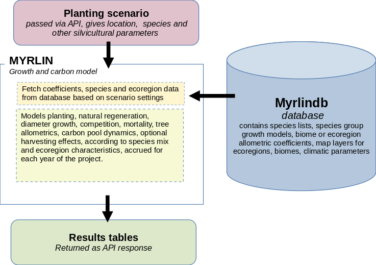
The model retrieves all necessary species and ecoregion data, including growth model and allometric coefficients from the database, and then proceeds through an annual cycle of simulating growth, mortality, regeneration, and necromass changes. These results are accrued as tables and returned to the calling program, where they can be interpreted and presented via a user interface.

Biomes, ecoregions and project location

MYRLIN uses the widely accepted system of WWF global biomes and ecoregions^[6]^[7]. These map the world into large scale vegetation-climate complexes (biomes), subdivided into phytogeographic realms, and further subdivided into distinctive mosaics of animal and plant species (ecoregions). The project location is mapped to one or more ecoregions (if the site is near an ecoregion boundary). The applicable ecoregions and biomes are then used to select the coefficients and factors for the various equations in the model.

Figure 2 : Interactive map of global biomes, realms and ecoregions

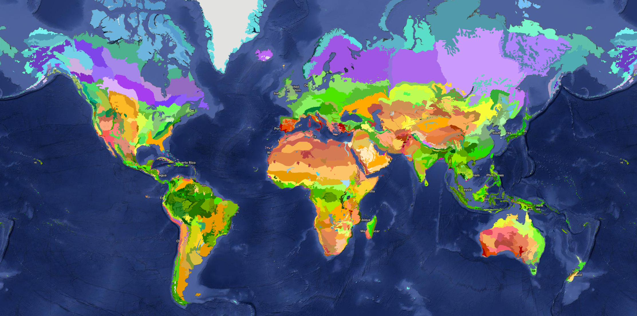
Information on biome and ecoregion affects several aspects of model performance:

Species are tagged with the ecoregions in which they occur. Different suitability indices will be selected according to whether they are in a native ecoregion , a biome in which that ecoregion occurs, or a foreign biome. This selects a suitability factor that affects growth and mortality rate.
Coefficients other than those which are species-related are specified according to biomes, so that different multipliers and factors may be applied. For example, some allometry factors are relative to biome.
Maximum biomass, net primary production, root:shoot ratios and other allometries are compiled by ecoregion as database tables from global studies and research compilations^[8]^[9]^[10]^[11]. These are therefore adapted to the specific ecoregions of the project and conform to IPCC Tier 2 or Tier 3 standards^[12].

Planting, regeneration and growth potential

MYRLIN is a cohort model^[13] in which trees of the same species and similar characteristics are represented as a cohort. Cohort models have many of the characteristics of individual tree models, but are more efficient at the analytical representation of stochastic processes, and are scale-independent, equally able to represent 1 or 10,000 ha of forest. A cohort in MYRLIN is defined as having the following common characteristics:

Species
Growth potential
Age
Tree diameter
Tree height
Crown status
Stocking (Trees per km²)

Cohorts are created at the time of tree planting, or during stand development, through natural regeneration. For each species planted or regenerating naturally, a frequency distribution of cohorts is created, which represent variation in natural growth potential due to genetics and local environment. The growth potential is a multiplier applied to diameter increment and remains constant for the life of the cohort.

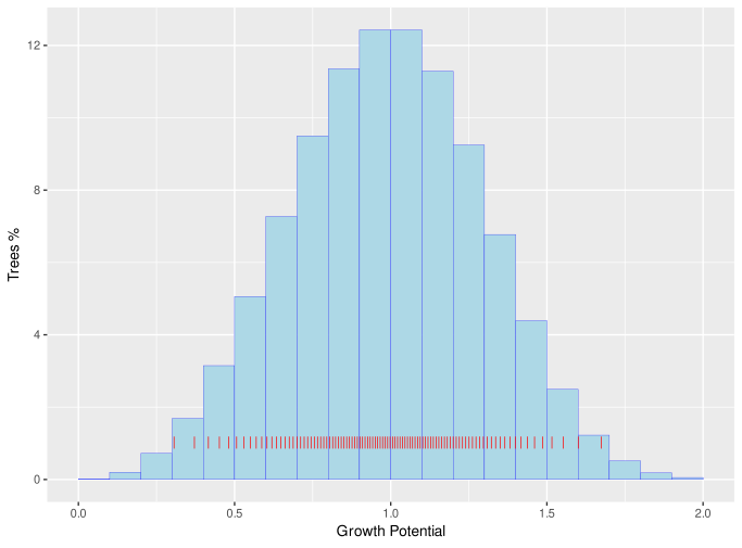
Growth potential values are assigned from a Weibull distribution with shape parameter of 3.6, which is symmetric and similar to a normal distribution^[14]. Figure 3 shows the distribution of cohort growth potentials with a scale parameter of 1.

Figure 3 : Distribution of cohort growth potential

The Weibull function in its cumulative form is expressed by the equation:

{eq.1} $P = 1 - exp(-(x/\alpha)^\beta)$

where P is probability of a value less than or equal to x, $\alpha$ is the scale parameter and $\beta$ the shape parameter. When creating cohorts from this distribution, cohorts with equal stem numbers are created, but with growth potential defined by the inverse equation:

{eq.2} $x_i = \alpha(-ln(1-P_i))^{(1/\beta)}$

Here $x_i$ is the growth potential of the i'th cohort and $P_i$ is the cumulative proportion of the stocking up to and including that cohort. The red lines on the above figure show the distribution of $x_i$ when 100 cohorts, each with 1% of total stocking, are generated at planting.

During the life of the simulated forest, cohort age, diameter, height, crown status, and stocking are updated. Species and inherent growth potential remain invariable. If due to mortality or harvesting, stocking declines to zero, then the cohort is extinguished. New cohorts are created by planting, re-stocking and natural regeneration. Figure 4 illustrates the sequence of these processes, which are described in detail in the following sections.

Figure 4 : Flowchart of the MYRLIN model

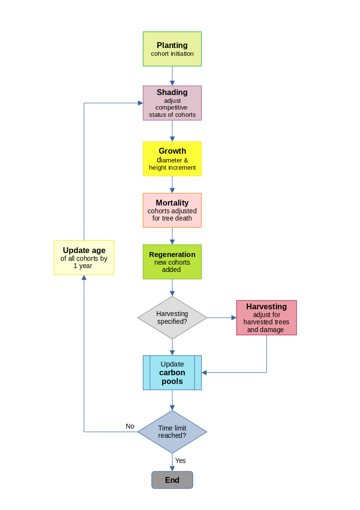
As well as being created at the time of planting or regeneration, cohorts may split, as a result of competition leading to a change in the crown status of part of a cohort. They may also be merged, if all the parameters except stocking converge to within a small limit. This maintains the efficiency of the simulation by reducing the total number of cohorts, which can become large with long and complex sumulations.

Diameter growth

Tree diameter growth under natural forest conditions is highly variable from year to year and tree to tree, but clearly influenced by species, competitive status and tree size and age^[15]. In most cases, detailed data to construct growth models are lacking, and species in the database therefore are mostly grouped by common characteristics of typical mature size, ecological type (pioneer, light demanding, shade tolerant, etc) and assigned to MYRLIN groups with standardised growth patterns. However, where data or models exist for well-studied species, such as Eucalyptus or Tectona (Teak), these can be individually assigned. In general, diameter growth is calculated as:

{eq.3} $D_{k}^{*} = D_{k,t} + \Delta D_k$

{eq.4} $\Delta D_k = f_m(D_k, A_k, C_k).g(B).S$

where:

$D_{k}$ is the diameter of cohort $k$ at the start of the growth period (year)
$D_{k}^{*}$ is the diameter of cohort $k$ at the end of the growth period
$\Delta D_k$ is diameter increment, or growth, for cohort k
$f_m()$ is the MYRLIN group growth model for the species of that cohort
$A_k$ is the age of cohort k
$C_k$ is the competitive status of cohort k
$g(B)$ is a function of total biomass B that tends to 0 as B tends to ecoregion limiting biomass
$S$ is a multiplier used to adjust for site quality, defaulting to 1 for a normal site.

Mortality

Mortality, or the death of trees, is a normal process during stand development. MYRLIN includes the following mortality factors:

(1) Planting or early mortality

This occurs usually in the first 2-3 years after planting, when the seedlings are more vulnerable to predators, drought and ground fires. The model requires the user to specify a period over which planting mortality occurs (typically 1-3 years) say $t$ , and the total percentage losses expected from this factor, say $M$ . Then the annual mortality rate (AMR), say $m_{pl}$ , during the planting period is given by:

{eq.5} $m_{pl} = 1 - (1-M)^{1/t}$

This is applied to all cohorts whose age is within the period of planting mortality, including cohorts that are created by natural regeneration or re-stocking, as these are subject to similar vulnerabilities.

(2) Mortality due to competition or shading

Trees which become shaded and suppressed during growth of the stand will die more rapidly. This will happen when the energy required for respiration exceeds that produced by photosynthesis over a period of months or years. The rate at which this happens is a species characteristic related to their shade tolerance.

In even-aged, uniform plantations, or young stands of re-growth forest, it is known as the stem exclusion stage of stand development^[16]. It follows the Reineke or self-thinning line^[17], a logarithmic relation between tree numbers and mean diameter. In mixed forest with many species and age classes, the relationship is less exact, but data shows there are still clear limits on the numbers of trees above a given diameter that can exist on a site.

In MYRLIN this is modelled by applying differential mortality factors according to competitive status, so that mortality rate is a logarithmic function of competitive status. If $C_k$ is the competitive status of a tree, scaled such that 0 indicates free-growing or dominant trees, and 1 are deeply-shaded trees, then mortality from shading is given by:

{eq.6} $m_{sh} = \alpha C_k^{\beta}$

Here, $\alpha$ and $\beta$ are coefficients that depend on the MYRLIN group of the species.

During their life-span trees will be attached by various fungi and diseases, which may cause death diretcly or may weaken them so they become more prone to wind breakage or fire damage. An attribute of the MYRLIN group, or growth model for the species, is the typical mature size of the tree, ( $D_{95}$ ), or 95% percentile of the cumulative diameter distribution. Once the tree has reached this size, a regular age-related mortality rate is applied in addition.

Tree Height

Tree height is determined from tree diameter, stand basal area and biome, using the equations of Feldpausch et al (2012)^[18]. This usage is in preference to the equations of Chave et al (2014)^[19] as they have been found to be more accurate in the tropical regionsbased on local allometry, particularly reflecting the effect of stand density on the height-diameter relationship^[20]^[21]. The Feldpausch equation is:

{eq.7} $h = \exp(\beta_0 + \beta_1. ln(d) + \beta_2. G)$

where the $\beta_i$ are coefficients specific to the biome and realm, $h$ is estimated tree height in metres, $d$ is tree diameter at 1.3 m in cm, and $G$ is the stand total basal area in m2/ha.

However, outside the biomes covered by Feldpausch's data, namely in temperate and boreal regions, especially in conifer-dominated forests, the Chave equation is better supported and is therefore used in these biomes. It has with the following form:

{eq.8} $h = \exp(\beta_0 + \beta_1.E + \beta_2.ln(d) + \beta_3.ln(d)^2)$

where the $\beta_i$ are coefficients which differ between broadleaf and conifers, E is an Environmental stress coefficient determined for the location^[22], summarised in the database by ecoregions.

Competition

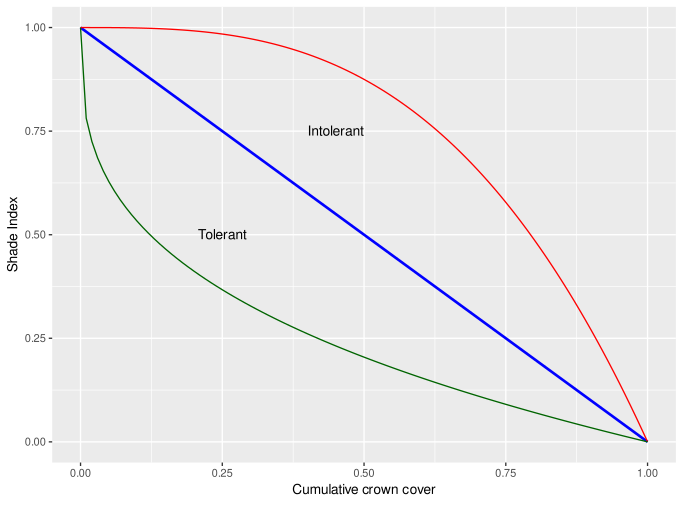
A competition index $C_k$ between 0 and 1 is assigned to each cohort at the beginning of each growth period (see Figure 4). This is calculated by first sorting the cohorts from smallest to largest by diameter, and then calculating the cumulative crown cover for each cohort relative to the total. Crown projection area is based on the allometric equations of Jucker et al (2017)^[23], with the form:

{eq.9} $A = \frac{\pi}{4}.10^{-4}\space [\exp(\beta_0 + \beta_1.ln(d) + \beta_2.\zeta)]^2$

where $A$ is the crown projection area in m of a tree of $d$ cm dbh, $b_i$ are coefficients, and $\zeta$ (zeta) is either 0 for broadleaf species (angiosperms), or 1 for conifers and palms. Cumulative crown cover $\upsilon_k$ for the k'th cohort is then given by:

{eq.10} $\upsilon_k = \displaystyle \frac{\Sigma_{i=1}^{k}A_i.N_i}{\Sigma_{i=1}^{m}{A_i.N_i}}$

where $A_i$ , $N_i$ are the crown projection area and the number of trees in the i'th cohort, and $m$ is the total number of cohorts. The cumulative crown cover is then modifed according to the relative shade tolerance for the species or MYRLIN group in the k'th cohort, according to the expression:

{eq.11} $C_k = 1 - \upsilon_k^\tau$

where $\tau$ (tau) is tolerance, $C_k$ is the competition or shading index, from 0 (no shading) to 1(fully shaded). The $\tau$ value is adjusted for best fit for species if growth data if this is available, but otherwise uses biome default values. Figure 5 shows how the adjustment between the cumulative crown cover and the shading index will look for these values (Green $\tau=1/3$ ; Blue $\tau=1$ ; Red $\tau=3$ ; ).

Figure 5 : Adjustment of competition index according to shade tolerance

Harvesting

Harvesting is currently allowed as a simple percentage of trees to be removed, applied systematically to all size classes. A starting year for harvesting is given as an option. Once that year has been reached, the designated proportion, say $L$ , is removed periodically every felling cycle. For each cohort k, the stocking after harvest $N_a$ is therefore:

{eq.12} $N_{a,k} = N_k.(1-L)$

and the harvested stems are given by:

{eq.13} $N_{h,k} = N_k.L$

The harvesting process, no matter how carefully planned or executed, inevitably causes extensive damage to the residual stand, with post-logging mortality that extends over several years ^[24] ^[25]. For MYRLIN, the ratio of damaged stems to stems harvested is given as a biome-specific parameter referred to as mortality due to logging $m_L$ . Equation 12 is therefore modified to include this effect, so that the remaining stocking becomes:

{eq.14} $N_{a,k} = N_k.[(1-L) - (L.m_L)]$

whilst the number of trees killed or damaged in the cohort $N_{m,k}$ is given by:

{eq.15} $N_{m,k} = N_k.L.m_L$

Typically $m_L$ will have a value of around 1 in humid tropical forest. In other words, for every tree removed, one of similar size will be killed or damaged sufficiently severely that it will die within 1-2 years. However, in other biomes these ratios may be less. Open woodlands for example, will have much lower rates of damage, whilst coniferous forests also generally allow lower rates of damage depending on the type of harvesting.

The harvested trees $N_{h,k}$ will be used to calculate biomass of products $B_p$ and the necromass of residues $M_r$ from branchwood and logging waste. The logging damage also contributes directly to the necromass pool $M_r$ .

A consequence of harvesting, and the associated logging damage (which includes, for example, skid trails and loading areas) is that the forest canopy is opened up and the ground disturbed. This encourages regeneration, particularly of the more light demanding and pioneer-type species. Using equation 9, with $A_k$ being the per tree crown projection for cohort k, $N_k$ as the stocking per cohort before harvesting, and $N_{a,k}$ being stocking after harvesting (from equation 14), the proportion of canopy opening $R_o$ is calculated as:

{eq.16} $R_o = \displaystyle 1 - \frac{\Sigma(A_k.N_{a,k})}{\Sigma({A_k.N_k})}$

From this equation, if there are no trees left after harvesting, $R_o$ will be 1 (100% canopy opening), whilst if the harvesting is very light, the canopy opening will likewise be small. The natural regneration function is applied as described in the relevant section above to the open areas created by harvesting and associated site disturbance.

This version of the harvesting model is intended to simulate light selection felling under continuous cover forestry. It can also simulate heavy periodic fellings applied across the whole project area. However, it is not designed to emulate patch clear-felling whereby, for example, 3.3% of an area is clearfelled each year over a 30-year cycle. For this, some adjustments to the model will be required. The harvesting also does not consider bias in stem selection towards larger or smaller trees. These features will be added to later versions of the model.

Roundwood timber volumes from the harvesting are added to the product carbon pool. Currently product pools are not usually admissable for carbon credits, and so are not considered in detail.

Carbon Pools

Figure 6 : Carbon pool dynamics

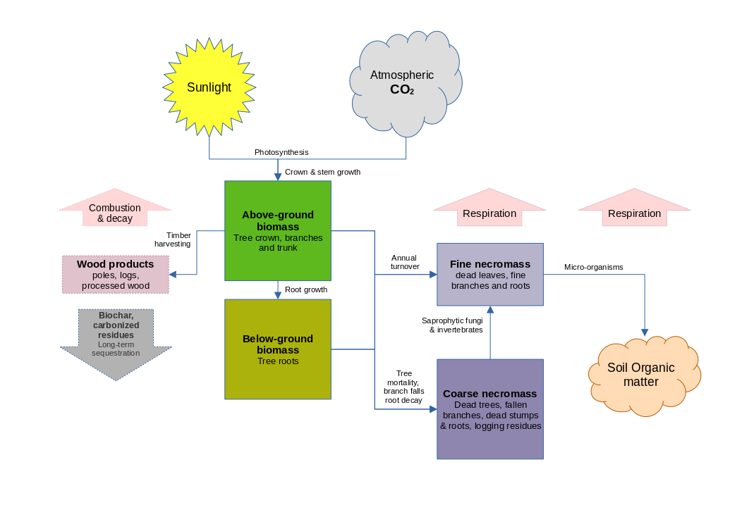
Figure 6 shows the main carbon-pools and processes. Not all of these are included in the present version of MYRLIN. The model is focussed on the biomass and necromass carbon pools. Soil organic matter and the more detailed analysis of the product pool are not included. The process of growth, whereby atmospheric CO₂ and soil H₂O (water) are converted to complex polysaccharides such as cellulose and lignin via photsynthesis, is modelled empirically using the functions described in the foregoing sections. The forest growing stock is described in the model as cohorts of species, diameter, and tree numbers. Their above-ground and below-ground biomass are calculated from these via the allometric equations described in the next sections. Accumulation rates for leaves and fine roots to the fine necromass pool are estimated from published data according to biome. This pool may typically be around 5% of total sequestered carbon. Coarse necromass from dead trees and branch falls can amount to some 15% of the total, and may increase markedly after harvesting for 1-2 decades due to damage and residues. Both these pools have annual decay rates, and material moves from the coarse to the fine necromass pools as a result of the activity of small invertebrates and fungi. Fine necromass is finally incorporated as soil organic matter (SOM) through a web of micro-organisms under normal, aerobic conditions. However, in permanently waterlogged or frozen soils, necromass may not fully breakdown and can accrue as peat. All these pools also lose CO₂ to the atmosphere through respiration, as well as possibly, annual or periodic fires. Peat deposits may be decomposed if conditions are changed through drainage or climate change.

Above-ground biomass

Above-ground biomass of a cohort, $B_{a,k}$ is calculated for each cohort k from diameter $d_k$ , wood density $\rho_k$ and Environmental Stress $E$ using the function of Chave et al (2014)^[19:1]:

{eq.17} $B_{a,k} = \exp(\beta_0 + \beta_1.E + \beta_2.ln(\rho_k) + \beta_3.ln(d_k) + \beta_4.ln(d_k)^2)$

The $d_k$ diameter values are given for each cohort. Wood density $\rho_k$ is looked up in the database for the species of cohort k. Environmental stress values are given by Chave et al (op. cit.) and have been computed in the database as average values for each ecoregion. Total above-ground biomass for the forest is calculated from the above as:

{eq.18} $B_{a} = \Sigma( B_{a,k}.N_k)$

where $N_k$ is the stocking (trees per ha) of the k'th cohort.

Root:shoot ratios and total biomass

Total biomass is estimated using a root:shoot ratio (RSR). The RSR is the ratio of root to above-ground biomass. A global map of root:shoot ratios compiled from current research^[11:1] has been used to derive RSR average values for each ecoregion. If $B_t$ is total biomass and $R_e$ the average root:shoot ratio for the ecoregion, then the relation is:

{eq.19} $B_t = B_a.(1 + R_e)$

Forest necromass : Deadwood and litter

The necromass pool is initially assumed to be zero for a planted site, and accrues dead material from tree mortality and litterfall (leaf turnover). If harvesting occurs, additional dead material will accrue from the stumps of harvested trees, residues after logging such as branchwood and trimmings and accentuated mortality due to tree damage and ecological changes. Material is lost from necromass due to respiration to CO₂ by saprophytic organisms as it decays to soil organic matter. If the total number of trees dying from all sources in cohort k during a year is $N_{d,k}$ then equations (17)-(19) can be applied to the dead trees to estimate accrued necromass.

The decay rate of necromass is given as a half-life ( $\lambda$ , lambda) for each biome, looked up from the database. Using $M$ to symbolize total necromass at the start of a period, $\Delta M$ as accrued necromass from natural mortality and harvesting during the period, and $M^*$ as final necromass at the end of the year, we will have:

{eq.20} $M^* = (M + \Delta M) . e^{(-ln(2)/\lambda))}$

The term $e^{(-ln(2)/ \lambda))}$ represents the proportion of the carbon pool remaining after 1 year if the decay half-life is $\lambda$ years. For example, with a 10-year half-life, the proportion remaining after one year is 93.3%. We can note that 0.933¹⁰ is 0.5, indicating that after 10 years, half would remain.

Output Tables

MYRLIN generates three output tables in its current version: (1) Carbon pools, (2) Forest growing stock and (3) Growing stock broken down by species. The content of each of these is illustrated for a simple example in the sections below. Only values for every 5'th year are shown for brevity, but MYRLIN produces annual tables up to the specified limit of the simulation. These examples are based on a mixture of Khaya anthotheca, Markhamia lutea and Isoberlinia scheffleri planted in equal proportions at 1600 trees per ha (2 x 3 m spacing) in the Eastern Arc ecoregion of Tanzania, but the format of the tables is independent of the species mix.

Table of carbon pools

This output shows the main carbon pools in tons CO₂ per ha for each year of the simulation. This table is the one of primary interest for carbon credit estimation.

trees is the above ground biomass in woody trees and shrubs (the model does not include biomass of grasses or herbs).
roots is below ground biomass, or tree roots.
necromass is total carbon sequestered in deadwood, coarse and fine litter, but not including soil organic matter.
total is the sum of the above three pools, or total sequestered carbon.
seqpy is carbon sequestered per year.

 year   trees  roots necromass   total  seqpy
    0   1.983  0.496     0.252   2.731  2.731
    5  88.339 22.085     8.663 119.087 28.627
   10 182.566 45.641    31.388 259.595 26.114
   15 249.534 62.384    54.122 366.040 17.784
   20 298.757 74.689    67.072 440.519 13.715
   25 340.208 85.052    76.564 501.823 11.810
   30 377.422 94.355    84.631 556.408 10.556

This table therefore shows that by year 30, this forest has accrued 556 tCO₂ ha^-1, of which 68% is above-ground biomass, 17% is tree roots, and 15% is necromass. The sequestration rate peaks in year 5 at 28.6 tCO₂ ha^-1 yr^-1 and has declined by year 30 to 10.6 tCO₂ ha^-1 yr^-1.

Table of aggregate forest growing stock

The forest growing stock table is mainly of interest for silviculture, forest management, and also model verification. The statistics shown in this table are as follows:

nha Trees per hecatare.
dbh Quadratic mean diameter of all trees, in cm. (Quadratic mean diameter is also known as the diameter of the tree of mean basal area). As is conventional in forestry, tree diameter (dbh) is measured at 1.3 m above ground.
hdom Dominant height in m, or mean height of the 100 largest diameter trees per ha. This is a good indicator of canopy height, and is a conventional forestry metric.
ba Basal area, or sum of the cross sectional areas of the trees at 1.3 m height, in m² ha^-1.
vol Total wood volume, in m³ ha^-1. Extractable or commercial timber volume is likely to be around 60-70% of this figure.
volh Harvested volume, in m³ ha^-1. This is roundwood volume, before any conversion factors to sawn volume is applied, but excludes an allowance for residues such as branchwood and defective sections. In this example, no harvesting is assumed, so it is zero.
D0-D100 Trees numbers per ha by diameter classes. D0 are trees 0-4.99 cm dbh, D5 are trees 5-9.99 cm, etc. D100 includes all trees of 100 cm dbh and above.

 year     nha   dbh  hdom    ba     vol volh      D0     D5    D10    D20    D30 ...  
    0 1600.00  2.63  4.41  0.87   2.508    0 1557.33  42.67   0.00   0.00   0.00  
    5 1387.85 12.28 13.93 16.45 114.413    0  147.92 644.50 428.64 166.79   0.00  
   10  937.96 19.10 21.44 26.88 247.032    0   31.69 125.06 253.82 146.44 123.05 
   15  844.52 22.07 26.61 32.30 343.992    0    7.57  27.98  72.64  86.84  79.06 
   20  568.36 28.27 30.28 35.67 413.552    0    1.60   7.92  10.27  70.97  41.87 
   25  427.00 33.81 33.35 38.33 471.217    0  146.68  58.72  13.58  37.38  37.11 
   30  447.11 33.94 35.95 40.45 522.706    0  113.78 110.54  38.29  21.16  25.86

The table shows that by year 30, there will be 447 trees remaining, from an inital planting of 1600 trees ha^-1. They will have a mean diameter of 34 cm, a dominant height of 36 m, and represent 523 m³ ha^-1 of timber.

Table of growing stock by species

The species growing stock table has the same columns as the aggregate forest table, except that, for simplicity, diameter class breakdown is not shown. However, all statistics are per species. This table can be used to understand the relative dynamics of species performance, as some will be faster growing, shorter lived, whilst other slower growing, long-lived species will eventually dominant the forest. The fast growing species are important for establishing early crown cover and suppression of unwanted plants such as grasses, and also give earlier, more rapid carbon sequestration. The longer-lived, slower growing species maintain the process of carbon sequestration as the short-lived species start to senesce, and also contribute importantly to plant and animal biodiversity and habitat creation.

The columns in the table, where they differ from the forest growing stock table above, are as follows:

locid This combines with spp to give a database-wide unique species list, and identifies the origin of the several lists that have been combined.
spp This is a mnemonic species code, used with locid as a database lookup key.
nha, dbh, ba, vol, volh are as defined for the forest table, but only pertainng to the particular species.
lhm is Lorey's mean height, defined as $\frac{\Sigma d^2.h}{\Sigma d^2}$ , with h being tree height and d being diameter^[26]. This gives an indication of the mean height of the dominant trees of that species, and is used instead of hdom, as defined above, because dominant height is not a definable metric for a single species in a diverse mixture.

 year locid spp    nha   dbh   lhm    ba     vol volh
    0     2 ISS 533.33  1.73  2.35  0.13   0.257    0
    0     2 KHA 533.33  3.66  3.83  0.56   1.839    0
    0     2 MAR 533.33  2.07  2.64  0.18   0.412    0
    5     2 ISS 458.82  7.29  7.04  1.92   9.257    0
    5     2 KHA 488.29 17.68 12.35 11.99  91.787    0
    5     2 MAR 440.74  8.57  7.76  2.54  13.369    0
   10     2 ISS 257.52  8.06 10.13  1.31   7.678    0
   10     2 KHA 451.20 25.75 19.15 23.50 225.846    0
   10     2 MAR 229.24 10.71 11.56  2.07  13.507    0
   15     2 ISS 239.49  5.99 13.15  0.67   4.585    0
   15     2 KHA 419.99 30.42 24.33 30.52 331.179    0
   15     2 MAR 185.05  8.69 14.72  1.10   8.227    0
   20     2 ISS 160.28  6.48 16.04  0.53   4.069    0
   20     2 KHA 301.85 38.04 28.36 34.31 402.695    0
   20     2 MAR 106.23  9.97 17.16  0.83   6.788    0
   25     2 ISS 124.35  8.16 15.94  0.65   4.802    0
   25     2 KHA 230.45 45.15 32.04 36.89 459.954    0
   25     2 MAR  72.20 11.82 17.82  0.79   6.461    0
   30     2 ISS 139.71  8.77 15.58  0.84   5.997    0
   30     2 KHA 217.97 47.63 35.61 38.84 510.591    0
   30     2 MAR  89.43 10.44 17.92  0.77   6.118    0

In the above example, KHA is Khaya anthotheca, a large long-lived tree; MAR is Markhamia lutea, smaller and of shorter life span, whilst ISS is Isoberlinia scheffleri, of intermediate size. It can be seen that by year 30, the initial stock of Markhamia (MAR) has declined much more than the other species, both due to earlier senescence, and competition and shading from the taller trees. The smaller trees are indeed, essentially dominanted by the Khaya, but nonetheless provide an important biodiversity and protective role, as young Khaya grown in pure stands would otherwise likley be susceptible to Hypsipyla outbreaks^[27].

Conclusion

This documentation describes the logic and empirical basis for the MYRLIN forest model in its current state of development (version 0.5003 of April 2024). It will be updated as the model evolves. Currently in process are the following extensions:

The database of species is being updated according to project demand.
Input of baseline data from sample plots in existing forests and woodlands is being enabled.
Soil organic matter, wetland, peat soils and mangrove carbon dynamics are being added.
Modelling of product carbon pools, including biochar, timber and other wood products will be extended.
Modelling of herbs and grasses will be included in addition to woody biomass.

Additionally, growth models and allometry are being continuously reviewed in the light of latest research and carbon market standards and requirements. Any updates will be included in this documentation as they are implemented.

Bibliography

Wright, HL; Alder, D [Ed.] (2000) Humid and semi-humid tropical forest yield regulation with minimal data. Workshop proceedings, CATIE, Costa Rica, 5-9 July 1999. Oxford Forestry Institute Occasional Papers 52. 95 pp. ↩︎
Alder, D; Oavika, F; Sanchez, M; Silva, , JNM; Van der Hout, P; Wright, HL. (2002) A comparison of species growth rates from four moist tropical forest regions using increment-size ordination. International Forestry Review 4(3)196-205. https://bio-met.co.uk/pdf/ifr2002.pdf ↩︎
Alder, D (2020) Updating the MYRLIN models for growth projection in mixed tropical forest. Consultancy Report, FAO, Rome, 25 pp.https://bio-met.co.uk/pdf/FAO-Myrlin-Feb-2020-Report.pdf ↩︎
Alder, D (2019) Evolving MYRLIN for sustainable management of Mixed Tropical Forests in the 2020s. Talk given at FAO, Rome, 14 November 2019 ↩︎
IPCC (2006) Guidelines for National Greenhouse Gas Inventories : Volume 4: Agriculture, Forestry and Other Land Use - Chapter 4 Forest Land.. http://www.ipcc-nggip.iges.or.jp/public/2006gl/vol4.html. ↩︎
Olson, DM; Dinerstein, E; Wikramanayake, ED; et al (2001) Terrestrial ecoregions of the world: a new map of life on Earth. Bioscience 51(11):933-938. https://doi.org/10.1641/0006-3568(2001)051[0933:TEOTWA]2.0.CO;2 ↩︎
Dinerstein, E; David Olson, D; Joshi, A; et al (2017) An ecoregion-based approach to protecting half the terrestrial realm. BioScience 67: 534–545, https://academic.oup.com/bioscience/article/67/6/534/3102935 ↩︎
Susan C. Cook-Patton, Sara M. Leavitt, David Gibbs, et al. (2020) Mapping carbon accumulation potential from global natural forest regrowth. Nature 585 (24 Sep 2020) 545-550. https://doi.org/10.1038/s41586-020-2686-x. ↩︎
Zheng, D.L., S.D. Prince, and R. Wright (2013) NPP Multi-Biome: Gridded Estimates for Selected Regions Worldwide, 1954-1998, R3. ORNL DAAC, Oak Ridge, Tennessee, USA. https://doi.org/10.3334/ORNLDAAC/614. ↩︎
ESA (2021) CCI Biomass Product User Guide v3. Online document: ESA Climate Change Initiative - BIOMASS project 2020, https://climate.esa.int/media/documents/D4.3 CCI PUG V3.0 20210707.pdf. ↩︎
Yuanyuan Huang, Phillipe Ciais, Maurizio Santoro (2021) A global map of root biomass across the world’s forests. Earth Syst. Sci. Data, 13, 4263–4274, https://doi.org/10.5194/essd-13-4263-2021. ↩︎ ↩︎
IPCC (2019) 2019 Refinement to the 2006 IPCC Guidelines for National Greenhouse Gas Inventories, Volume 4: Agriculture, Forestry and Other Land Use, Chapter 3: Consistent Representation of Lands. https://www.ipcc-nggip.iges.or.jp/public/2006gl/pdf/4 Volume4/V4 03 Ch3 Representation.pdf. ↩︎
Vanclay, JK (1994) Modelling of Growth and Yield of Tropical Moist Forests. CAB International, Wallingford. 312 pp. http://espace.library.uq.edu.au/eserv/UQ:8211/ModellingForestG.pdf. ↩︎
Bailey, RL; Dell, TR (1973) Quantifying diameter distributions with the Weibull function. Forest Science 19(2)97-104. ↩︎
Alder, D (1995) Growth modelling for mixed tropical forests. Department of Plant Sciences, University of Oxford. Tropical Forestry Paper 30, 231 pp. https://ora.ox.ac.uk/objects/uuid:0390f933-b42e-4342-856b-8ebe81517968 ↩︎
Oliver, CD; Larson, BC (1990) Forest Stand Dynamics. McGraw-Hill Inc., New York. 467 pp. ↩︎
Pretzsch, Hans; Biber, Peter (2005) A Re-Evaluation of Reineke's Rule and Stand Density Index. Forest Science 51(4)304-320. https://bio-met.co.uk/pdf/an1055.pdf ↩︎
Feldpausch, TR; Banin, L; Phillips, OL; et al (2011) Height-diameter allometry of tropical forest trees. Biogeosciences, 8, 1081–1106, https://doi.org/10.5194/bg-8-1081-2011, 2011. ↩︎
Chave, J; Réjou-Méchain, M; Burquez, A; et al. (2014) Improved allometric models to estimate the above-ground biomass of tropical trees. Global Change Biology 20: 3177-3190, DOI: 10.1111/gcb.12629. https://bio-met.co.uk/pdf/an1164.pdf ↩︎ ↩︎ ↩︎
Alder, D (2020) An analysis of the Fiji National Forest Inventory 2006 and Permanent Sample Plot measurements 2010-2018 - Part 1 : Fiji National Forest Inventory 2006. Consultancy Report to Ministry of Forestry, Fiji , October 2020, 40 pp. https://bio-met.co.uk/pdf/an1232.pdf. ↩︎
Masota, AM; Zahabu, E; Malimbwi, RE, Bollandsas, OM; Eid, TH (2014) Volume models for single trees in tropical rainforests in Tanzania. Journal of Energy and Natural Resources 3(5) 66-76. ↩︎
The global raster map of Environmental Stress^[19:2] values can be downloaded from http://chave.ups-tlse.fr/pantropical_allometry.htm in various formats. ↩︎
Jucker, T; Caspersen, J, Chave, J; et al. (2017) Allometric equations for integrating remote sensing imagery into forest monitoring programmes. Global Change Biology (2017) 23, 177–190, doi: 10.1111/gcb.13388. https://onlinelibrary.wiley.com/doi/full/10.1111/gcb.13388 ↩︎
Bertault, JG; Sist, P (1995) The effects of logging in natural forests.. Bois et Forets des Tropiques. 1995, No. 245, 5-20; 8 ref. https://www.researchgate.net/publication/230660891_The_effect_of_logging_in_natural_forests ↩︎
Jonkers, WBJ (1987) Vegetation structure, logging damage and silviculture in a tropical rainforest in Surinam. Wageningen Agricultural University, Ph.D. thesis, 172 pp. https://research.wur.nl/en/publications/vegetation-structure-logging-damage-and-silviculture-in-a-tropica ↩︎
Thomas B. Lynch, Robert F. Wittwer, Douglas J. Stevenson, Michael M. Huebschmann, A Maximum Size-Density Relationship between Lorey's Mean Height and Trees per Hectare, Forest Science, Volume 53, Issue 4, August 2007, Pages 478–485, https://doi.org/10.1093/forestscience/53.4.478 ↩︎
E. Opuni-Frimpong, D.F. Karnosky, A.J. Storer, E.A. Abeney, J.R. Cobbinah (2008) Relative susceptibility of four species of African mahogany to the shoot borer Hypsipyla robusta (Lepidoptera: Pyralidae) in the moist semideciduous forest of Ghana. Forest Ecology and Management,Volume 255, Issue 2, 2008, Pages 313-319. https://doi.org/10.1016/j.foreco.2007.09.077. ↩︎